Example Usage
The data used in the following examples are simulated using OpenAI’s ChatGPT. Identifiable fields (full names, addresses, etc.) are also simulated.
Using Extracts (> clean_REDCap)
First, we can use a (.csv) extract of the data and data dictionary from REDCap:
dat_raw <- read.csv(file = "materials/miscellaneous/DemoRSyntheticData_DATA_2025-03-18_0728.csv")      # Read in the data
dict    <- read.csv(file = "materials/miscellaneous/DemoRSyntheticData_DataDictionary_2025-03-18.csv", # Read in the data dictionary
                    check.names = FALSE ## So spaces, punctuation etc. are preserved in tibble
                    )
Visualising the first few rows of our data:
head(dat_raw, n = 10) %>%
  thekids_table(line_spacing = 0.8,
                padding = 1.5)
#> Warning in check_font_family(font_family = font_family, fallback_family =
#> fallback_font_family): Font 'Barlow' not found; falling back to 'sans'.
record_id |
form_1_complete |
demo_title |
demo_fname |
demo_dob |
demo_address |
demo_postcode |
anthro_sex |
anthro_weight |
anthro_height |
assess_iq |
demo_edu |
demo_income |
demo_num_dep |
med_hist_cvd |
med_hist_diabetes |
life_pol |
life_house_date |
life_super |
synthetic_1_complete |
|---|---|---|---|---|---|---|---|---|---|---|---|---|---|---|---|---|---|---|---|
1 |
0 |
Mr. |
William Moore |
1990‑01‑24 |
99 St Georges Terrace, Scarborough, WA |
6006 |
Male |
97.7 |
1.56 |
58 |
3 |
0 |
2 |
0 |
1 |
Liberal |
1999‑04‑05 |
4458703 |
0 |
2 |
0 |
Mr. |
William Brown |
1998‑10‑24 |
6011 |
Other |
62.3 |
1.53 |
54 |
1 |
0 |
1 |
0 |
1 |
Central |
1985‑05‑31 |
14636346 |
0 |
|
3 |
0 |
Mr. |
Elizabeth Williams |
1983‑03‑01 |
87 Hay Street, Joondalup, WA |
6011 |
Male |
146.0 |
2.02 |
119 |
3 |
4 |
6 |
1 |
0 |
Liberal |
5334516 |
0 |
|
4 |
0 |
Ms. |
John Miller |
1985‑02‑13 |
85 Hay Street, Perth CBD, WA |
6006 |
Female |
66.4 |
1.53 |
54 |
2 |
0 |
5 |
0 |
1 |
Labour |
1989‑11‑13 |
6399928 |
0 |
5 |
0 |
Mr. |
John Brown |
1973‑12‑10 |
33 Beaufort Street, Mount Lawley, WA |
6005 |
Other |
114.9 |
1.55 |
57 |
3 |
0 |
6 |
1 |
1 |
Labour |
1985‑12‑02 |
294741 |
0 |
6 |
0 |
Ms. |
Michael Williams |
1997‑01‑29 |
24 St Georges Terrace, Northbridge, WA |
6011 |
Female |
69.2 |
1.64 |
69 |
3 |
1 |
2 |
0 |
0 |
Labour |
1992‑04‑19 |
10847340 |
0 |
7 |
0 |
Ms. |
Michael Davis |
1990‑10‑10 |
84 Hay Street, Northbridge, WA |
6007 |
Male |
85.6 |
2.03 |
121 |
3 |
4 |
5 |
1 |
0 |
Labour |
1991‑04‑28 |
6320541 |
0 |
8 |
0 |
Mx. |
Mary Brown |
1994‑08‑20 |
85 Murray Street, Mount Lawley, WA |
6008 |
Male |
76.7 |
1.70 |
77 |
3 |
1 |
1 |
0 |
0 |
Central |
2009‑03‑12 |
1726473 |
0 |
9 |
0 |
Ms. |
Michael Taylor |
1978‑05‑13 |
29 King Street, Fremantle, WA |
6008 |
Other |
109.8 |
66 |
1 |
0 |
0 |
0 |
1 |
Liberal |
2004‑03‑05 |
14534640 |
0 |
|
10 |
0 |
Mx. |
Patricia Moore |
1990‑06‑06 |
76 Adelaide Terrace, Cottesloe, WA |
6012 |
Other |
139.8 |
1.93 |
107 |
1 |
3 |
7 |
0 |
0 |
Liberal |
1992‑12‑20 |
11706012 |
0 |
Similarly, we can visualise our standardised data dictionary extract from REDCap:
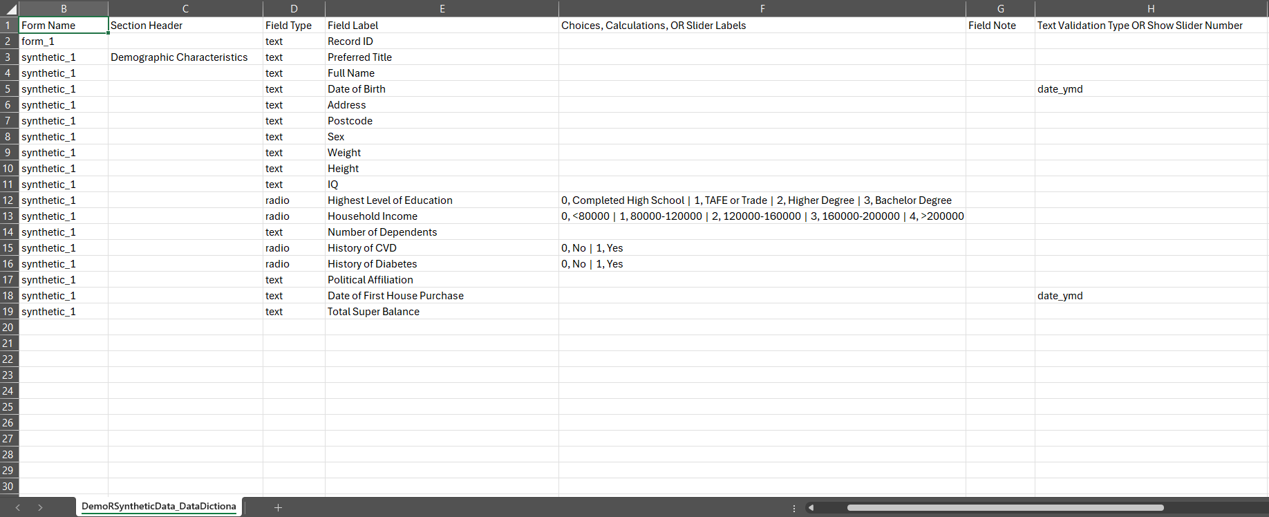
Clearly:
- Some categorical fields (
demo_income,demo_num_dep,med_hist_cvd,med_hist_diabetes) are numerically coded and will need resolution before proceeding. - Column headers are variable names, not labels.
If we were to tabulate this data (stratifying by, say,
med_hist_cvd), we must manually apply labels to categorical
variable levels (which is indeed made easier using
thekidsbiostats::fct_case_when) and variable names (passed
directly to tbl_summary):
dat_raw %>%
  select(demo_postcode, anthro_sex:life_pol, life_super) %>%
  mutate(demo_edu = fct_case_when(demo_edu == 0 ~ "Completed High School",
                                  demo_edu == 1 ~ "TAFE or Trade",
                                  demo_edu == 2 ~ "Higher Degree",
                                  demo_edu == 3 ~ "Bachelor Degree"),
         demo_income = fct_case_when(demo_income == 0 ~ "<80000",
                                     demo_income == 1 ~ "80000-120000",
                                     demo_income == 2 ~ "120000-160000",
                                     demo_income == 3 ~ "160000-200000",
                                     demo_income == 4 ~ ">200000"),
         across(c(med_hist_cvd, med_hist_diabetes), ~fct_case_when(. == 0 ~ "No",
                                                                   . == 1 ~ "Yes")),
         across(c(anthro_sex, life_pol), ~case_when(. == "" ~ NA,
                                                    TRUE ~ .))) %>%

  tbl_summary(by = med_hist_cvd,
              type = list(demo_postcode ~ "categorical"),
              digits = list(all_categorical() ~ c(0, 1)),
              label = list(demo_postcode     ~ "Postcode",
                           anthro_sex        ~ "Sex",
                           anthro_weight     ~ "Weight",
                           anthro_height     ~ "Height",
                           assess_iq         ~ "IQ",
                           demo_edu          ~ "Highest level of education",
                           demo_income       ~ "Household income",
                           demo_num_dep      ~ "Number of dependents",
                           med_hist_diabetes ~ "History of diabetes",
                           life_pol          ~ "Political affiliation",
                           life_super        ~ "Total superannuation balance")
              ) %>%
  modify_spanning_header(all_stat_cols() ~ "**History of CVD**") %>%
  thekids_table()
#> Warning in check_font_family(font_family = font_family, fallback_family =
#> fallback_font_family): Font 'Barlow' not found; falling back to 'sans'.
#> Factor levels (in order): Completed High School, TAFE or Trade, Higher Degree, Bachelor Degree
#> Factor levels (in order): <80000, 80000-120000, 120000-160000, 160000-200000, >200000
#> Factor levels (in order): No, Yes
#> Factor levels (in order): No, Yes
#> 100 missing rows in the "med_hist_cvd" column have been
#> removed.
|
History of CVD |
|
|---|---|---|
Characteristic |
No |
Yes |
Postcode |
||
6000 |
72 (7.9%) |
69 (7.7%) |
6003 |
59 (6.5%) |
79 (8.8%) |
6004 |
85 (9.3%) |
81 (9.0%) |
6005 |
76 (8.3%) |
82 (9.2%) |
6006 |
89 (9.7%) |
90 (10.0%) |
6007 |
85 (9.3%) |
88 (9.8%) |
6008 |
85 (9.3%) |
88 (9.8%) |
6009 |
79 (8.6%) |
81 (9.0%) |
6010 |
82 (9.0%) |
78 (8.7%) |
6011 |
101 (11.1%) |
77 (8.6%) |
6012 |
101 (11.1%) |
83 (9.3%) |
Unknown |
46 |
44 |
Sex |
||
Female |
308 (33.7%) |
272 (30.6%) |
Male |
285 (31.2%) |
314 (35.3%) |
Other |
320 (35.0%) |
304 (34.2%) |
Unknown |
47 |
50 |
Weight |
107 (82, 129) |
106 (85, 129) |
Unknown |
46 |
47 |
Height |
1.79 (1.65, 1.96) |
1.81 (1.66, 1.96) |
Unknown |
44 |
52 |
IQ |
89 (69, 111) |
90 (70, 110) |
Unknown |
50 |
47 |
Highest level of education |
||
Completed High School |
216 (23.6%) |
215 (24.2%) |
TAFE or Trade |
234 (25.5%) |
219 (24.6%) |
Higher Degree |
218 (23.8%) |
230 (25.8%) |
Bachelor Degree |
249 (27.2%) |
226 (25.4%) |
Unknown |
43 |
50 |
Household income |
||
<80000 |
199 (21.7%) |
183 (20.6%) |
80000-120000 |
176 (19.2%) |
169 (19.0%) |
120000-160000 |
186 (20.3%) |
189 (21.3%) |
160000-200000 |
182 (19.9%) |
162 (18.2%) |
>200000 |
173 (18.9%) |
186 (20.9%) |
Unknown |
44 |
51 |
Number of dependents |
3 (2, 5) |
3 (1, 5) |
Unknown |
51 |
45 |
History of diabetes |
471 (51.3%) |
467 (52.6%) |
Unknown |
41 |
53 |
Political affiliation |
||
Central |
301 (33.3%) |
309 (34.3%) |
Labour |
270 (29.9%) |
325 (36.0%) |
Liberal |
332 (36.8%) |
268 (29.7%) |
Unknown |
57 |
38 |
Total superannuation balance |
7,456,367 (3,930,725, 11,271,067) |
7,679,442 (3,868,717, 11,056,757) |
Unknown |
42 |
53 |
1n (%); Median (Q1, Q3) | ||
The above code chunk is clearly quite sizeable and required a significant degree of user input.
Instead, using clean_REDCap:
dat_mod <- clean_REDCap(d = dat_raw,
             dict = dict,
             yesno_to_bool = T)

dat_mod %>%
  select(demo_postcode, anthro_sex:life_pol, life_super) %>%

  tbl_summary(by = med_hist_cvd,
              type = list(demo_postcode ~ "categorical"),
              digits = list(all_categorical() ~ c(0, 1))
              ) %>%
  modify_spanning_header(all_stat_cols() ~ "**History of CVD**") %>%
  thekids_table()
#> Warning in check_font_family(font_family = font_family, fallback_family =
#> fallback_font_family): Font 'Barlow' not found; falling back to 'sans'.
#> 100 missing rows in the "med_hist_cvd" column have been
#> removed.
|
History of CVD |
|
|---|---|---|
Characteristic |
No |
Yes |
Postcode |
||
6000 |
72 (7.9%) |
69 (7.7%) |
6003 |
59 (6.5%) |
79 (8.8%) |
6004 |
85 (9.3%) |
81 (9.0%) |
6005 |
76 (8.3%) |
82 (9.2%) |
6006 |
89 (9.7%) |
90 (10.0%) |
6007 |
85 (9.3%) |
88 (9.8%) |
6008 |
85 (9.3%) |
88 (9.8%) |
6009 |
79 (8.6%) |
81 (9.0%) |
6010 |
82 (9.0%) |
78 (8.7%) |
6011 |
101 (11.1%) |
77 (8.6%) |
6012 |
101 (11.1%) |
83 (9.3%) |
Unknown |
46 |
44 |
Sex |
||
47 (4.9%) |
50 (5.3%) |
|
Female |
308 (32.1%) |
272 (28.9%) |
Male |
285 (29.7%) |
314 (33.4%) |
Other |
320 (33.3%) |
304 (32.3%) |
Weight |
107 (82, 129) |
106 (85, 129) |
Unknown |
46 |
47 |
Height |
1.79 (1.65, 1.96) |
1.81 (1.66, 1.96) |
Unknown |
44 |
52 |
IQ |
89 (69, 111) |
90 (70, 110) |
Unknown |
50 |
47 |
Highest Level of Education |
||
Completed High School |
216 (23.6%) |
215 (24.2%) |
TAFE or Trade |
234 (25.5%) |
219 (24.6%) |
Higher Degree |
218 (23.8%) |
230 (25.8%) |
Bachelor Degree |
249 (27.2%) |
226 (25.4%) |
Unknown |
43 |
50 |
Household Income |
||
<80000 |
199 (21.7%) |
183 (20.6%) |
80000-120000 |
176 (19.2%) |
169 (19.0%) |
120000-160000 |
186 (20.3%) |
189 (21.3%) |
160000-200000 |
182 (19.9%) |
162 (18.2%) |
>200000 |
173 (18.9%) |
186 (20.9%) |
Unknown |
44 |
51 |
Number of Dependents |
3 (2, 5) |
3 (1, 5) |
Unknown |
51 |
45 |
History of Diabetes |
471 (51.3%) |
467 (52.6%) |
Unknown |
41 |
53 |
Political Affiliation |
||
57 (5.9%) |
38 (4.0%) |
|
Central |
301 (31.4%) |
309 (32.9%) |
Labour |
270 (28.1%) |
325 (34.6%) |
Liberal |
332 (34.6%) |
268 (28.5%) |
Total Super Balance |
7,456,367 (3,930,725, 11,271,067) |
7,679,442 (3,868,717, 11,056,757) |
Unknown |
42 |
53 |
1n (%); Median (Q1, Q3) | ||
The variable levels and labels are automatically applied.