Function | Description |
|---|---|
clean_REDCap | Cleans REDCap data exports by applying factor levels and converting column classes per a REDCap data dictionary. |
create_project | Creates a folder structure for a new project, as well as an R Project file and basic R scripts. Example. |
create_template | Creates a Quarto document from one of several template (extention) choices. Example. |
fct_case_when | Like dplyr::case_when but the output variable is of class factor, ordered based on the order entered into the case_when statement. Example. |
round_df | Rounds all numeric columns in a data frame or tibble, preserving trailing zeroes. Example. |
round_vec | Rounds all values in a vector, preserving trailing zeroes. Example. |
scale_color_thekids | ggplot scale_color theme for applying “The Kids”-themed colours. |
scale_fill_thekids | ggplot scale_fill theme for applying “The Kids”-themed colours. |
thekids_model | Generates a collection of informative model output in a structured list when provided data and model specification. Example. |
thekids_model_output | Generates a collection of informative model output in a structured list when provided with an existing model object. |
thekids_table | Creates a formatted flextable with “The Kids” themed colours and fonts. Example. |
thekids_theme | Applies “The Kids” theme to a ggplot object, including colours, fonts and changes to other elements for a cleaner look. Example. |
theme_institute | Like thekids_theme, but for historical projects completed using the Telethon Kids Institute style guide. |
Overview
We created a package!
A major attraction of the R programming language is its vast library of free packages, which can be found on both CRAN (the Comprehensive R Archive Network) or hosted on other sites such as GitHub. These packages can provide ready-made functions, datasets and/or templates for all kinds of applications (some staggeringly niche). In the field of statistics and data analysis, it is rare to encounter any methodology, model and/or algorithm which has not also been implemented somewhere in some R package.
Packages can also be easily developed for use within teams or individual use, to automate or simplify tasks which appear often.
What does thekidsbiostats do?
In summary, the package provides:
- Functions to automate and/or simplify regular/routine tasks in our workflow.
- Functions and Quarto templates which apply consistent formatting and theming to documents, ggplots, tables, etc.
A complete list of functions, with brief descriptions, is found in the table below. The rest of this post will provide some worked examples for many of the functions in this list.
How to Install the Package
The package (and all of its code!) are available here: https://github.com/The-Kids-Biostats/thekidsbiostats.
If you would like to follow along with the examples below, simply run the code below:
remotes::install_github("https://github.com/The-Kids-Biostats/thekidsbiostats")

library(thekidsbiostats)
Examples
Helper Functions
create_project
This is the first function called when we begin a new project. It creates a folder structure based on parameters it is given, and an R Project file. The real power of this function comes from the ext_name parameter, which allows various templates (or ‘extensions’) to be used for the project. So far, we have a ‘basic’ extension and a ‘targets’ extension (which adds files and folders used by the targets package). Other extensions are in the works for specific types of projects.
Upon calling create_project(), a pop-up will appear allowing the user to choose where the new project should be located:
create_project(project_name = "package_demo", ext_name = "targets",
               docs = F)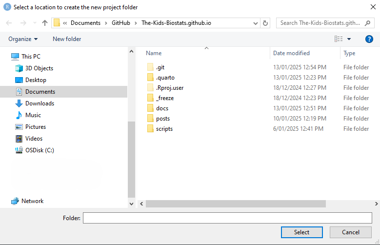
In this instance, we create a project called “package_demo”. Both the project directory and the R project (.Rproj) file take this name. We choose the “targets” extension, which means our directory starts with a “_targets.R” file and a “scripts” folder (had we chosen the “basic” extension, neither of these objects would be created).
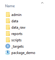
Additionally, the function has the data, data-raw, admin, reports and docs parameters. These can be set to either TRUE or FALSE to include these folders in the project directory or not (default for all is TRUE). Note that we set “docs” to FALSE and so it does not appear in our directory above.
The “reports” directory created by create_project() is the default location for Quarto templates to be placed when calling create_template(), which we look at now…
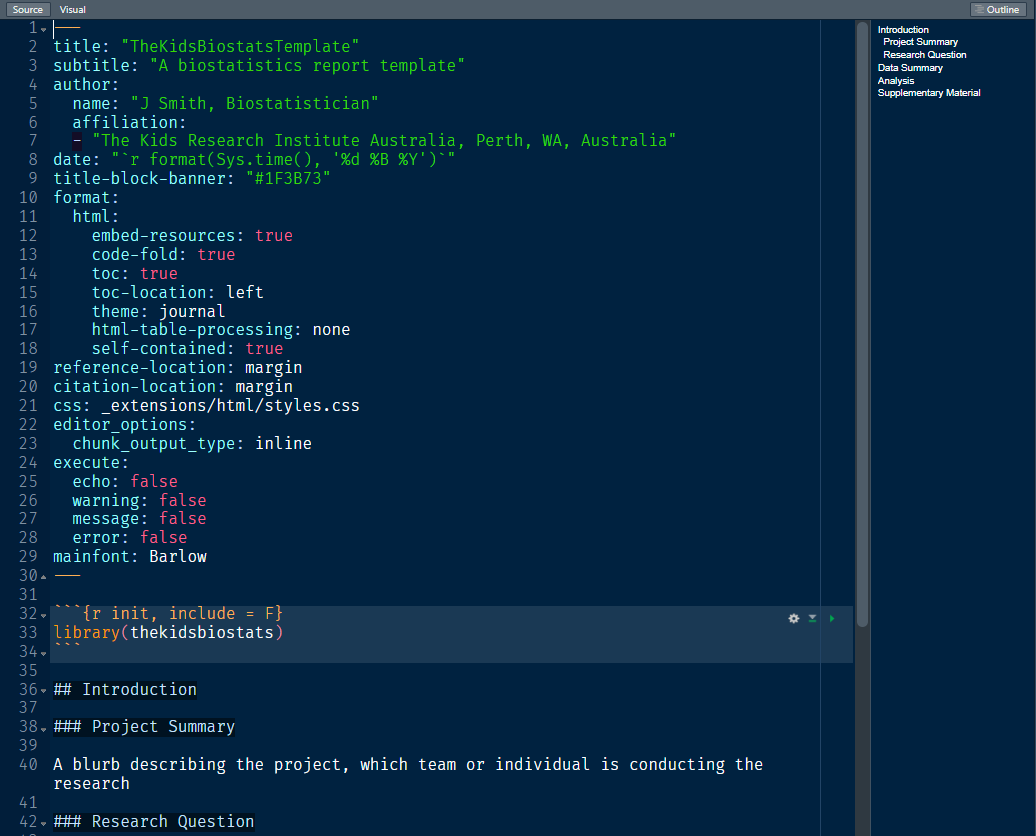
create_template
The purpose of create_template() is to generate ready-to-populate Quarto templates with “The Kids styling” already applied. Two templates are possible using the ext_name parameter: html and word, corresponding to the report format that we desire.
We can call it below, telling it to create the document in the “package_demo/reports” folder we created using create_project() above.
create_template(file_name = "demo_report", directory = "package_demo/reports/")The resulting quarto document looks like this:
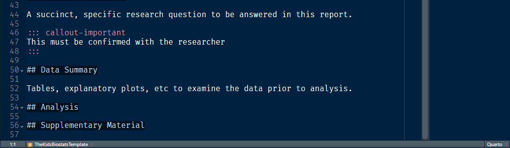
And rendered:
thekids_model
We have a dedicated post exploring the use of thekids_model.
Briefly, this function provides a standardised list of outputs for commonly used models in R. This includes the model itself, diagnostics, marginal means, and clean tables of typical model output (coefficients, confidence intervals, p-values etc). The above blog post details exactly how to display these nicely in a Quarto html document.
round_vec and round_df
These two functions are examples where the sole purpose is keep code concise and to the point. Often when we present figures whether it is in plots, tables or in written form, we wish to preserve trailing zeroes when rounding numbers to a x decimal places.
Below we demonstrate the difference between the base R round() and round_vec() when rounding to decimal places.
original | round | round_vec |
|---|---|---|
1.8003 | 1.8 | 1.80 |
1.9998 | 2 | 2.00 |
2.5812 | 2.58 | 2.58 |
round_vec() consistently has 2 decimal places, whereas round() drops any trailing zeroes, which is often undesirable for presentation.
round_df() can be called on a data frame or tibble to round every numeric column in that object at once.
fct_case_when
In a similar vein to the above function, fct_case_when is essentially dplyr::case_when but with one handy addition: the resulting vector is a factor where the levels are ordered in the same order they are defined within the case_when statement.
The factor levels are the result of the default case_when() function combined with as.factor(), and are simply ordered alphabetically.
x <- 1:50
case_when(
  x %% 35 == 0 ~ "fizz buzz",
  x %% 5 == 0 ~ "fizz",
  x %% 7 == 0 ~ "buzz",
  TRUE ~ "everything else"
) %>% as.factor %>% levels
[1] "buzz" "everything else" "fizz" "fizz buzz" In comparision, fct_case_when() orders the factor levels based on the order of their appearance in the argument:
x <- 1:50
thekidsbiostats::fct_case_when(
  x %% 35 == 0 ~ "fizz buzz",
  x %% 5 == 0 ~ "fizz",
  x %% 7 == 0 ~ "buzz",
  TRUE ~ "everything else"
) %>% levels
[1] "fizz buzz" "fizz" "buzz" "everything else"Theming
Using functions that automatically apply a set of formatting options to plots and tables saves time, allowing us to focus on the analysis and interpretation. Code also looks a lot cleaner when those 10 lines of ggplot per plot are automated away. Importantly, these functions also ensure a polished and consistent appearance across our team, so that output looks the same irrespective of who generated it.
thekids_theme
The thekids_theme() function applies consistent theming to ggplot2 visualizations. It uses a clean, minimal aesthetic with fonts and colors that align with The Kids branding. Here’s an example of a plot before themeing:
ggplot(mtcars, aes(x = mpg, y = wt, col = factor(cyl))) +
  geom_point(size = 3) +
  labs(x = "Miles per Gallon", y = "Weight", col = "Cylinders")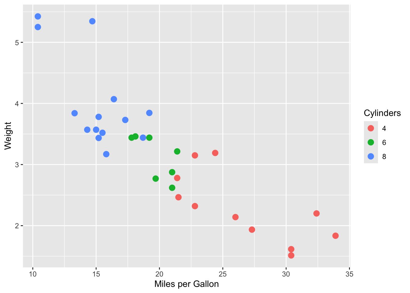
ggplot(mtcars, aes(x = mpg, y = wt, col = factor(cyl))) +
  geom_point(size = 3) +
  labs(x = "Miles per Gallon", y = "Weight", col = "Cylinders") +
  thekids_theme()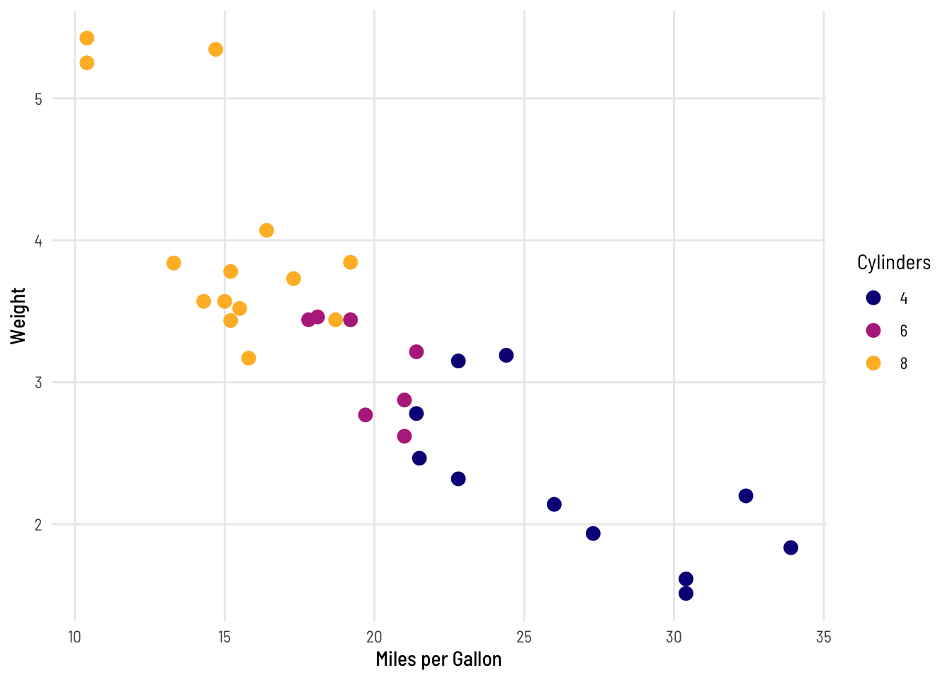
thekids_table
thekids_table() produces tables styled with The Kids branding and is powered by the flextable package. This includes by default applying the Barlow font, compact formatting (our preference!), and zebra-striping for readability, though these can all be altered/disabled via parameters.
For example, a raw table output from the mtcars dataset looks like this:
head(mtcars, 5) mpg cyl disp hp drat wt qsec vs am gear carb
Mazda RX4 21.0 6 160 110 3.90 2.620 16.46 0 1 4 4
Mazda RX4 Wag 21.0 6 160 110 3.90 2.875 17.02 0 1 4 4
Datsun 710 22.8 4 108 93 3.85 2.320 18.61 1 1 4 1
Hornet 4 Drive 21.4 6 258 110 3.08 3.215 19.44 1 0 3 1
Hornet Sportabout 18.7 8 360 175 3.15 3.440 17.02 0 0 3 2Now, applying thekids_table() transforms it into a clean, visually appealing format with branding elements:
head(mtcars, 5) %>%
  thekids_table(colour = "Saffron", font.size = 10)
mpg | cyl | disp | hp | drat | wt | qsec | vs | am | gear | carb |
|---|---|---|---|---|---|---|---|---|---|---|
21.0 | 6 | 160 | 110 | 3.90 | 2.620 | 16.46 | 0 | 1 | 4 | 4 |
21.0 | 6 | 160 | 110 | 3.90 | 2.875 | 17.02 | 0 | 1 | 4 | 4 |
22.8 | 4 | 108 | 93 | 3.85 | 2.320 | 18.61 | 1 | 1 | 4 | 1 |
21.4 | 6 | 258 | 110 | 3.08 | 3.215 | 19.44 | 1 | 0 | 3 | 1 |
18.7 | 8 | 360 | 175 | 3.15 | 3.440 | 17.02 | 0 | 0 | 3 | 2 |
This outputs a compact, zebra-striped table ready for inclusion in Word or HTML reports. However, the padding and striped options can be changed if we would prefer some more space without any stripes:
head(mtcars, 5) %>%
  thekids_table(colour = "Saffron", font.size = 10, padding = 4, striped = F)
mpg | cyl | disp | hp | drat | wt | qsec | vs | am | gear | carb |
|---|---|---|---|---|---|---|---|---|---|---|
21.0 | 6 | 160 | 110 | 3.90 | 2.620 | 16.46 | 0 | 1 | 4 | 4 |
21.0 | 6 | 160 | 110 | 3.90 | 2.875 | 17.02 | 0 | 1 | 4 | 4 |
22.8 | 4 | 108 | 93 | 3.85 | 2.320 | 18.61 | 1 | 1 | 4 | 1 |
21.4 | 6 | 258 | 110 | 3.08 | 3.215 | 19.44 | 1 | 0 | 3 | 1 |
18.7 | 8 | 360 | 175 | 3.15 | 3.440 | 17.02 | 0 | 0 | 3 | 2 |
Both thekids_theme() and thekids_table provide a host of options via parameters given to the functions.
Conclusions
The thekidsbiostats package significantly simplifies repetitive tasks, standardises formatting, and speeds up workflows. While tailored for use at The Kids Research Institute Australia, many of its features can be readily adapted to other contexts, providing a ready-to-go framework for data analysis and reporting.
There are plenty of arguments we didn’t go other in the this post, however they are all described in the documentation.
We hope you’ll give the package a try and find some or all of the functions useful in your own workflow. Please feel free to contact us at biostatistics@thekids.org.au (or raise an issue on our Github repository) if you encounter any bugs or would like to suggest additional features for any of our functions.
Acknowledgements
Thanks to Matt Cooper, Zac Dempsey and Elizabeth McKinnon for providing feedback on and reviewing this post.
AI Usage Note
The majority of this post and code were produced by the author. AI tools were used to refine the structure and wording.
Reproducibility Information
To access the .qmd (Quarto markdown) files as well as any R scripts or data that was used in this post, please visit our GitHub:
https://github.com/The-Kids-Biostats/The-Kids-Biostats.github.io/tree/main/posts/
The session information can also be seen below.
sessionInfo()R version 4.3.3 (2024-02-29)
Platform: aarch64-apple-darwin20 (64-bit)
Running under: macOS Sonoma 14.4.1
Matrix products: default
BLAS: /Library/Frameworks/R.framework/Versions/4.3-arm64/Resources/lib/libRblas.0.dylib
LAPACK: /Library/Frameworks/R.framework/Versions/4.3-arm64/Resources/lib/libRlapack.dylib; LAPACK version 3.11.0
locale:
[1] en_US.UTF-8/en_US.UTF-8/en_US.UTF-8/C/en_US.UTF-8/en_US.UTF-8
time zone: Australia/Perth
tzcode source: internal
attached base packages:
[1] stats graphics grDevices utils datasets methods base
other attached packages:
[1] kableExtra_1.4.0 thekidsbiostats_0.0.1 flextable_0.9.7
[4] gtsummary_2.0.4 extrafont_0.19 Hmisc_5.2-1
[7] lubridate_1.9.4 forcats_1.0.0 stringr_1.5.1
[10] dplyr_1.1.4 purrr_1.0.2 readr_2.1.5
[13] tidyr_1.3.1 tibble_3.2.1 ggplot2_3.5.1
[16] tidyverse_2.0.0
loaded via a namespace (and not attached):
[1] gtable_0.3.6 xfun_0.50 htmlwidgets_1.6.4
[4] tzdb_0.4.0 vctrs_0.6.5 tools_4.3.3
[7] generics_0.1.3 cluster_2.1.8 pkgconfig_2.0.3
[10] data.table_1.16.4 checkmate_2.3.2 uuid_1.2-1
[13] lifecycle_1.0.4 farver_2.1.2 compiler_4.3.3
[16] textshaping_0.4.1 munsell_0.5.1 janitor_2.2.1
[19] snakecase_0.11.1 fontquiver_0.2.1 fontLiberation_0.1.0
[22] htmltools_0.5.8.1 yaml_2.3.10 Rttf2pt1_1.3.12
[25] htmlTable_2.4.3 Formula_1.2-5 pillar_1.10.1
[28] extrafontdb_1.0 openssl_2.3.1 rpart_4.1.24
[31] fontBitstreamVera_0.1.1 zip_2.3.1 tidyselect_1.2.1
[34] digest_0.6.37 stringi_1.8.4 labeling_0.4.3
[37] labelled_2.14.0 fastmap_1.2.0 grid_4.3.3
[40] ftExtra_0.6.4 colorspace_2.1-1 cli_3.6.3
[43] magrittr_2.0.3 base64enc_0.1-3 foreign_0.8-87
[46] withr_3.0.2 gdtools_0.4.1 scales_1.3.0
[49] backports_1.5.0 timechange_0.3.0 rmarkdown_2.29
[52] officer_0.6.7 nnet_7.3-20 gridExtra_2.3
[55] ragg_1.3.3 askpass_1.2.1 hms_1.1.3
[58] evaluate_1.0.3 haven_2.5.4 knitr_1.49
[61] viridisLite_0.4.2 rlang_1.1.4 Rcpp_1.0.14
[64] glue_1.8.0 xml2_1.3.6 svglite_2.1.3
[67] rstudioapi_0.17.1 jsonlite_1.8.9 R6_2.5.1
[70] systemfonts_1.1.0